Querying Datacubes
with WCPS

What to Find Here

This section answers the key question: How does datacube analytics work through high-level, low-coding queries with WCPS?

Big Earth Data Analytics demands “shipping the code to the data” – however: what type of code?
For sure not procedural code (such as C++ or python) which requires strong coding skills from users and developers and also is highly insecure from a service administration perspective. Rather, use some safe, high-level query language, which also enables strong server-side optimizations, including parallelization, distributed processing, and use of mixed CPU/GPU, to name a few.
Paving the way for this future-oriented perspective, OGC already in 2008 has standardized the Web Coverage Processing Service (WCPS) geo datacube analytics language which today is part of the WCS suite, linked in through the WCS Processing extension. Today, WCPS is being used routinely in Petascale operational datacube services, e.g., in the global EarthServer federation.

My First WCPS Query

A WCPS query has several parts, the two most important ones being the for and the return clauses. The for part serves to indicate the coverage objects we want to work with, and to tie them to a variable - a shorthand, if you will - for subsequent processing directives. Say, we want to inspect coverages A, B, and C in turn using variable $c as an iterator (we note in passing that such variables start with a $ symbol). This is written as:

for $c in ( A, B, C )

This is fine, but not complete, as after all it does not give us any result. We need to add a return clause where we state what we actually want to get back. The following "hello world" example returns 42 (assuming coverages A, B, and C exists on the server, otherwise adapt the name accordingly):

for $c in ( A, B, C )
return 42

Ahem, nothing impressive, admittedly: all we get back is 3 times the literal 42 as below - but hey, we need to start somewhere.

42
42
42

Oh, by the way, if the expression is completely self-contained, i.e.: does not reference any coverage object, you can leave out the for clause, just to mention:

return 42

Try it: This and the further examples you can readily try out in the WCPS sandbox of the Earth Datacube Playground. Just select the sample query from the menu at the bottom and hit execute.
Don't get surprised by extra noise like diagram>>. This prefix is just a hint for the client to render whatever is returned as either pure text display (prefix text>>), a diagram (prefix diagram>>), or an image representation (prefix image>>); without any prefix you are prompted for a storage location for the file received.

Not impressive, but a first sign of life. Oh, by the way, such a simple number is returned in ASCII as text. This can be printed or easily converted into any programming language's number representation. If you will, ASCII is the transfer encoding.

Note: As the knowledgeable reader may suspect already: yes, WCPS syntax in its structure tentatively is similar to FLWOR expressions in XQuery; this has enabled easy integration of XPath metadata expressions in WCPS 1.1 which heralds seamless integration of data and metadata queries.

Things get more complicated once we start extraction from coverages - as we all know there is a plethora of format encodings available, end everybody has their own favourite. Now WCPS is graceful on this and lets you select your personal preference. As long as the data allows this - the server will have a hard time encoding something 4D into PNG which is just made for 2D, so that won't work.

Understood, but how do we express our desired encoding format? Well, by applying an encode() function on the result wich the coverage output as first parameter and the encoding format as second parameter, indicated through its MIME type like "image/tiff" for GeoTIFF. Assuming we have a small 2D coverage (be careful, you really don't want to try this with a multi-Terabyte object!) this could read as follows:

for $c in ( A )
return encode( $c, "image/tiff" )

The above query would return one GeoTIFF file; had we indicated a list of say 3 coverages then we would get back 3 GeoTIFF files, one for each iteration.

Now we are ready to roll - let us inspect next how we can extract from coverages. After all, as mentioned, we would not want to download coverages which typically are Big Data, hence "too big to transport".

Combining Coverages: Data Fusion

Oh, by the way, the for clause can do even more for us: combining several coverages. This is achieved by listing several variable declarations in the for clause. For example, let us request a band ratio (more on that below) from bands stored in two separate coverages, say MODIS-nir and MODIS-red. Ignoring the processing magic in the return clause for now - we will address this below - we can establish fusion requests like the following:

for $nir in ( MODIS-nir ),
    $red in ( MODIS-red )
return encode( (unsigned int) 127*(($red-$nir)/($red+$nir)+1), "image/tiff" )

Generally speaking, for some lineup

for $x₁ in (X_1,1,X_1,2,...),
    $x₂ in (X_2,1,X_2,2,...),
    ...,
    $x_n in (X_n,1,X_n,2,...)
return f($x₁,$x₂,...,$x_n)

each combination of the $x_i,j is generated and evaluated in turn. This allows data fusion on an arbitrary number of coverages. As an example, this INSPIRE WCS service contains a 4-way fusion.

Coverage Expressions

At the heart of WCPS are coverage expressions - they actually perform the heavy lifting of Big Data Analytics. A rich set of operators is provided by the language, effectively covering some mileage of Tensor Algebra, up to about the Fast Fourier Transform). We start our tour with the most basic operation: coordinate-based extraction from a coverage.

Coverage Subsetting

The most immediate operation, subsetting, we know already from WCS trimming and slicing. In WCPS, notation is more compact: instead of the WCS SUBSET sequence subsetting in WCPS is enshrined in brackets, such as:

$c[ Lat(30:60), Long(40:60), date("2020-03-21") ]

Sequence of axes does not matter, as we have always indicate the name of the axis addressed. As with WCS, axes left out will be delivered uncut. Needless to say, the lower bound must not be higher than the upper bound.

Induced Operations

In so-called induced operations some operation which is known on pixels silently gets applied to all pixels simultaneously. The following example multiplies wo coverages, an image and a bitmask, pixelwise:

for $s in ( Sentinel2 ),
    $m in ( SentinelCloudMask )
return
  encode( $s * $m , "image/png" )

Any unary or binary function defined on the cell types qualifies for induced use, including all the well-known arithmetic, comparison, Boolean, trigonometric, and exponential/logarithmic operations, as well as case distinction.

Talking about case distinction, the following example performs a color classification of land temperature (note the null value 99999 which is mapped to white, see the query result in the figure right):

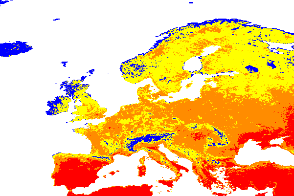
for $c in ( AvgLandTemp )
return
  encode(
    switch
      case $c = 99999 return {red: 255; green: 255; blue: 255}
      case $c < 18    return {red: 0; green: 0; blue: 255}
      case $c < 23    return {red: 255; green: 255; blue: 0}
      case $c < 30    return {red: 255; green: 140; blue: 0}
      default         return {red: 255; green: 0; blue: 0},
    "image/png"
  )

Expression Optimization: Leave it to the Server!

As always it is corageous to let the expression iterate over the full coverage. Being streetwise we therefore add subsetting:

for $c in ( AvgLandTemp )
return
  encode(
    switch
    case $c[ date("2014-07"), Lat(35:75), Long(-20:40) ] = 99999 return {red: 255; green: 255; blue: 255}
    case $c[ date("2014-07"), Lat(35:75), Long(-20:40) ] < 18    return {red: 0; green: 0; blue: 255}
    case $c[ date("2014-07"), Lat(35:75), Long(-20:40) ] < 23    return {red: 255; green: 255; blue: 0}
    case $c[ date("2014-07"), Lat(35:75), Long(-20:40) ] < 30    return {red: 255; green: 140; blue: 0}
    default                                                      return {red: 255; green: 0; blue: 0},
    "image/png"
  )

By instinct we have expressed the processing steps in the sequence that is most efficient: first subsetting, then pixel computations. However, things are getting unwieldy, repeating subset coordinates all over is onerous. We should not be forced to do it that way. Actually, a good optimizer, such as the one implemented in rasdaman, will rearrange automatically to the most efficient execution sequence. If we know that our WCPS server is that smart we can just as well indicate the subsetting once and for all at the end:

for $c in ( AvgLandTemp )
return
  encode(
    ( switch
        case $c = 99999 return {red: 255; green: 255; blue: 255}
        case $c < 18    return {red: 0; green: 0; blue: 255}
        case $c < 23    return {red: 255; green: 255; blue: 0}
        case $c < 30    return {red: 255; green: 140; blue: 0}
        default         return {red: 255; green: 0; blue: 0}
    ) [ date("2014-07"), Lat(35:75), Long(-20:40) ],
    "image/png")

Let Clause

And here is yet another way of making expressions crisper and easier to read: pulling parts out into separate variable definitions. This is what the let clause accomplishes by letting us give names to expressions; the above query would now read:

for $c in ( AvgLandTemp )
let $subset := [ date("2014-07"), Lat(35:75), Long(-20:40) ]
return
  encode(
    ( switch
      case $c = 99999 return {red: 255; green: 255; blue: 255}
      case $c < 18    return {red: 0; green: 0; blue: 255}
      case $c < 23    return {red: 255; green: 255; blue: 0}
      case $c < 30    return {red: 255; green: 140; blue: 0}
      default         return {red: 255; green: 0; blue: 0}
    ) [ $subset ],
    "image/png"
  )

Any number of variables can be defined, and it is highly recommended as it nicely structures queries for human eyes.

Multi-Band Constructor

Ready for a fun fact? We can construct entirely new coverages, cell-by-cell. We want to do this, for example, to support WebGL clients in doing 3D terrain draping. The trick is to provide a PNG image where RGB is built from some any source (like a satellite image) while feeding the alpha channel with the elevation data. Of course we will need to adjust resolution as both typically differ widely; we choose to re-scale the DEM. This is what the corresponding query looks like:

for $s in (SatImage),
    $d in (DEM)
return
  encode(
    struct {
      red:   $s.b7,
      green: $s.b5,
      blue:  $s.b0,
      alpha: scale( $d, 20 )
    },
    "image/png"
  )

Type Casting

In passing we note that also casts to different pixel types are available. This is necessary, for example, when some arithmetic operation would return float while the format (here: PNG) expects 8-bit unsigned quantities.

Note: The band ratio example above, if used for visualization, would likely need adjustment, too, as it returns float values between -1 and +1, not suitable for visual display. This illustrates the fact that WCS and WCPS primarily are data services, not visualization services - that said, visualization is a special case of queries where the result type is single- or three-band (sometimes, as we have seen, four-band) with 8-bit channel values. In general, data service delivering data that can be processed further, as opposed to WMS and WMTS which deliver images solely suitable for human consumption.

Coverage Constructor

In the functional, side-effect free language of WCPS we already have derived new coverages, to be shipped to the client in some encoding. What we have manipulated was the mostly pixel values. The domain set was either given by a subsetting expressions or carried over implicitly. The new range type, finally, was either forced by a cast or derived automatically, All these are special cases of a general constructor capable of building a completely new coverage with all elements controlled. This coverage constructor has three clauses. In the coverage section a name is given to the new coverage, in the over section the extent is defined for each axis the coverage will have, and in the values clause an expression is indicated for computing the coverage's cell values. Here is an example creating a 256x256 matrix with axes x and y containing a white-to-black grey bar:

coverage GreyMatrix
over     $px x ( 0 : 255 ),
         $py y ( 0 : 255 )
values   (char) ( ( $px + $py ) / 2 )

Should we want to refer to another coverage then this is no problem, in both domain and range set. Auxiliary function imageCrsDomain() delivers the extent for some axis, in Cartesian coordinates so that iteration is possible:

coverage GreyMatrix
over     $px x imageCrsDomain( $c, Long )
         $py y (imageCrsDomain( $c, Lat )
values   (char) ( ( $px + $py ) / 2 )

Coverage Condenser

What's missing still is some way to aggregate coverage values. In coverage speak this is said to condense values. Such a condenser function receives a coverage expression to iterate over and delivers min, max, sum, avg, count as well as some (is there any true value?) and all (are all values true?). For example, this below yields the maximum value in the red band of a satellite scene:

for $s in ( LandsatScene )
return max( $s.red )

Note that there is no encode() - the result, a single number, is simply returned as an ASCII string.

Very often condensers are used in conjunction with a coverage constructor. Here is an example, deriving a histogram from some satellite band:

for $s in ( LandsatScene )
return
  encode(
    coverage $bucket ( 0 : 255 )
    values count( $s.red = $bucket ),
    "text/csv"
   )

And just like there is a constructor generalizing induced operations there is also a general condenser construct behind these condenser functions, which now turn out to be special cases. The general structure is, in analogy to the constructor, the keyword condense followed by the operation to be executed, an over clause indicating the region to iterate over, and finally a using clause with an expression to be evaluated at each position. Hence, the above max() example is equivalent to the following writing:

for $s in ( LandsatScene )
return
  condense max
  over     $p in imageCrsDomain( $s )
  using    $s.red

So why should we use this much more complicated construct? Well, it has access to the coordinates, thereby allowing to express neighbourhood operations. This can be seen nicely when expressing a matrix multiplication (remember, it is a_i,k*b_k,j):

for $a in ( MatrixA ),
    $b in ( MatrixB ) 
return
  encode(
    coverage MatMult
    domain   $i in crsDomain($a)[0],
             $j in crsDomain($b)[1]
    values   condense +
             over     $k in crsDomain($a)[1]
             using    $a[ $i, $k ] * $b[ $k, $j ] ,
  "text/csv" )

Coverage Filtering

Sometimes we are interested in just some coverages, but we don't know upfront which of them qualify before we have seen their data contents. Downloading all candidates for client-side inspection is not an option as they are "too big to transport", so we need to let the server find out. This is accomplished with the where clause which performs server-side preselection among coverage sets by applying any criterion that you may provide; only thise coverages passing the filter will be forwarded to the return processing and delivery.

Here is an example that will give you the Bavaria DEM only if it contains heights over 3000m - which it doesn't, so the result will be empty (try with a smaller number!):

for $c in ( Bavaria_50_DSM )
where max( $c ) > 3000
return 1

A More Coverage Processing Example

Ready for a final effort? To show the expressive power of WCPS let us do edge detection using the Sobel oeprator given as

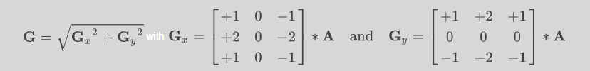
To WCPS this translates as:

for $c in (NIR)
let $kernel1 := coverage kernel1
                over     $x x (-1:1), $y y (-1:1)
                value list < 1; 0; -1; 2; 0; -2; 1; 0; -1 >,
    $kernel2 := coverage kernel1
                over    $x x (-1:1), $y y (-1:1)
                value list < 1; 2; 1; 0; 0; 0; -1; -2; -1 >,
    $cutOut := [ ${cutOut} ]
return
  encode(
    sqrt(
      pow(
        coverage Gx
        over $px1 i( imageCrsdomain( $c[$cutOut], i ) ),
             $py1 j( imageCrsdomain( $c[$cutOut], j ) )
        values
          condense +
          over     $kx1 x( imageCrsdomain( $kernel1, x ) ),
                   $ky1 y( imageCrsdomain( $kernel1, y ) )
          using    $kernel1[ x($kx1), y($ky1) ] * $c.${selectedBand}[ i($px1 + $kx1), j($py1 + $ky1) ] ,
        2.0
      )
      +
      pow(
        coverage Gy
        over $px2 i( imageCrsdomain( $c[$cutOut], i ) ),
             $py2 j( imageCrsdomain( $c[$cutOut], j ) )
        values
          condense +
          over     $kx2 x( imageCrsdomain($kernel2, x ) ),
                   $ky2 y( imageCrsdomain($kernel2, y ) )
        using    $kernel2[ x($kx2), y($ky2) ] * $c.${selectedBand}[ i($px2 + $kx2), j($py2 + $ky2) ] ,
        2.0
      )
    ),
    "image/jpeg"
  )

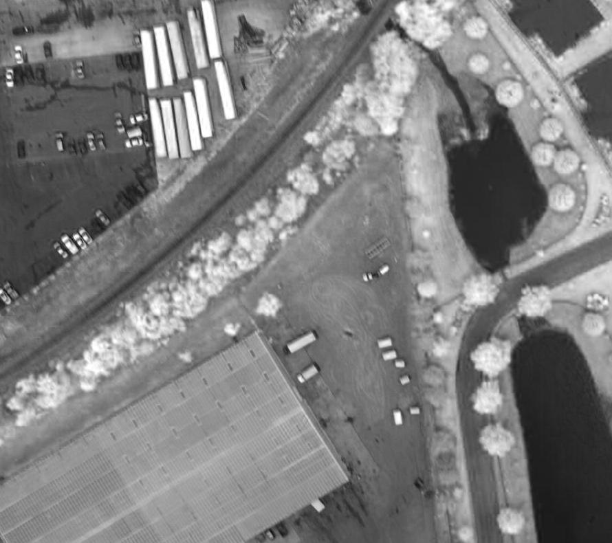
When applied in this demo to a false color image (left) the server returns this image (right):

Note: The WCPS syntax has been designed tentatively close to XQuery/XPath so as to allow integration with XML or JSON based metadata retrieval; Kakaletris et al have implemented a coupling of WCPS with XPath, leading to unified data/metadata queries, and the integrated data/metadata retrieval language WQS is prepared for this.

Finale: Sending the Request

Remains one mystery to be resolved: How is such a request sent to the server?

Basically, a query string can be transmitted a POST request. The GET variant has the advantage that the request can be sent as a single line even from a browser, but has the disadvantage that we need to URL-encode various characters that are not allowed to appear literally, such as spaces. While in common environments like JavaScript this is even done automatically we use the POST for demonstration through Linux command lines. The curl command is our friend here. It allows to specify both target URL and parameters, sends it to the server, and receives the result. Here is a working example:

curl 'https://ows.rasdaman.org/rasdaman/ows?service=WCS&version=2.0.1&request=ProcessCoverages' \
  -d 'query=for $c in (mean_summer_airtemp) return encode($c, "image/png")' -o wcps.png

The first parameter is the URL following the pattern of WCS, of which the ProcessCoverages request serving to send WCPS queries is a part. The -d parameter contains the query string, and the -o parameter finally determines the result file name.

That's All, Folks!

This concludes our primer on WCPS; for more introductory and detail information on various levels refer to the list below.

Articles & Links

Questions? Answers!

We gladly share our experience to answer any questions you may have, from strategic issues down to any technical depth. This can be discussed based on your own data, your own ecosystem requirements, and of course under strict confidentiality (such as under an NDA). Webinars as well as on-site meetings are possible.

Contact us - we gladly share our experience and insight from 20+ years of writing, implementing, and testing OGC, ISO, and INSPIRE standards, implementing them from Raspberry Pi to dozens-of-Petabytes archives.

High-Performance Datacube Engine:
rasdaman

The open-source pioneer datacube engine, rasdaman is OGC Coverages reference implementation.

The rasdaman engine has pioneered Actionable Datacubes® and Array Databases. With its enabling approach of a high-level datacube analytics language -- adopted into ISO SQL -- and underpinned by a po werful datacube architecture with federation, distributed data fusion, AI, highly effective query optimization, and more -- rasdaman remains the gold standard for modern multi-dimensional raster data services, being up to 74x faster than other engines.

Querying Datacubes with WCPS